How Ads Work - Part 2, Retrieval

Posted Feb 25, 2023 Updated Sep 14, 2024

13 min read

In the last post we looked at an overview of the entire Ads system. In this post we will talk about Retrieval in depth. To recap, in Retrieval the goal is to cast a wide net over the entire Ads Index and quickly select a few thousand ad candidates which are broadly relevant for the user and query context.

Text based document search
Graph Walks
Two Tower DNN
Indexing the Ads and Serving
Cold Start for new Ads
Closing Thoughts
Further Reading

In most Ads Serving systems, Retrieval is composed of several separate candidate generators. The results from several candidate generators are blended and rules (like ad budget) are used to further filter out candidates. Let’s take a look at some typical candidate generators.

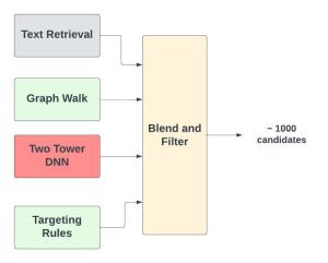Figure - Retrieval is composed of several candidate generators

Text based document search

This is traditionally how retrieval used to be done. The Ad is the document and the fields could be ad title, category and other inferred or explicitly set pieces of text. For search ads, the query is obviously the search query (possibly expanded with synonyms). The context and user can also be transformed to a text query by inferring the user’s category, interests and other attributes. Filters like targeting geography and other criteria can be easily applied in this setting.

Pros

Extremely mature and well established. Easy ways to do rule based selection like targeting for geography, broad user demographics, etc. Queries are blazingly fast thanks to data structures like the reverse index and postings list.
Fields in the document can be weighted to provide some level of tuning.
No cold start issues. No ML model trained on user interactions, so works for new ads and users

Cons

Does not learn from user interactions. There is no easy way to incorporate feedback in the form of user clicks, etc. Remember that in the end, we want to show ads that the user is likely to interact with.
Only text based. Ads usually have Images or Videos and Lucene like systems built around text tokens don’t handle these.
The field weights are usually set manually. Over time, these become a brittle black box that’s hard to maintain.

We will not go into details of Document based retrieval. This book is a great reference and the first few chapters are essential reading. The remarkable thing is that even in the Deep learning era, most retrieval systems do still use at least one Lucene like candidate generator.

Graph Walks

In social networks, users, advertisers and all other entities like brand or company pages can be thought of as nodes in a graph. Each edge represents some kind of interaction like following or friend-ing.

When we want to generate candidates for a particular user, we can do walks on this graph, starting from the user node and collecting a set of candidates as we explore the graph. This is a very flexible framework and we easily incorporate popularity (weights the edges and sample) and diversity (more breadth first exploration), etc

Pros

Graph based retrieval can offer a very different set of candidates that capture properties of the network structure.
Once the graph is built, it’s very fast to query.

I will add that DL techniques on Graphs like GraphSage that also account for additional features like text and visual representations can be thought of as Deep Learning extensions to this and are state of the art.

Two Tower DNN

This model was a major inflection point for recommender systems. Youtube published this paper and introduced the two tower model and it has now become the benchmark. We will take a good deep look at this model.

Problem Framing

Remember that our goal in retrieval is to select candidates that are likely to be interacted with. This leads to formulating it as a ML classification problem. For the youtube paper, it’s an extreme multi-class classification where the goal is to predict the next watched video. For Ads retrieval we can instead set it up as a simpler binary classification problem. A positive example is when a user clicks on an Ad. That’s the interaction we want. A negative example is all other cases (this gets interesting, read further for more details)

Model Structure

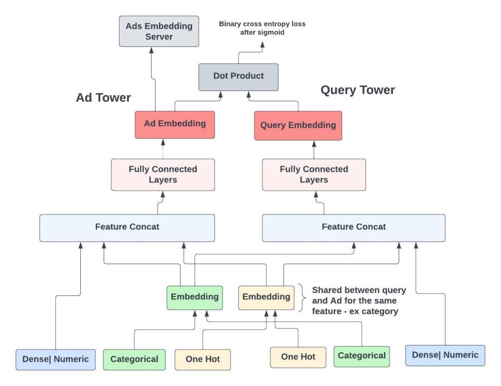Figure - The Two Tower DNN model

We separate out the model into two towers. The Ad tower and the Query . Keeping the towers separate is what allows fast retrieval during serving. We lose out on capturing more complex interactions between the Query and Ad, but remember our goal here is to have a lightweight model that gets us a good enough set of ad candidates.

The output of the top most layer in each tower is the embedding. A dot product between these L2-normalized embeddings is fed through a sigmoid to give a probability. The loss is then the standard binary cross entropy loss. Minimizing the loss leads to the Ad and Query embeddings getting closer together when the label is positive and further away when the label is negative.

The dimensionality of the bottom most layers depends on the input features. As we go higher up in each tower, the dimensions of the fully connected layers decrease and it’s typical for the top most embedding layer to have dimension 256 or lower. Note that this dimension has a direct impact on run time performance. The hidden layers are all ReLu. Regularization if required is usually just adding a few dropout layers.

Features and Preprocessing

It’s helpful to mentally group features into one hot, categorical, text, numeric and dense vector to better understand how preprocessing is done.

One Hot and categorical features are hashed into a fixed dimension vector and then fed into an embedding layer. This embedding layer can be shared between the Ad and Query tower. As an example consider the ad’s category which is a categorical feature. The user’s category can be inferred from past interactions. A single embedding layer for the category multi hot vector can be shared between the two towers, reducing the total number of model parameters.

Numerical features are normalized to be within a small range like [-1, 1] . Typically we use z-score normalization. If the distribution of the feature is heavily skewed, we can instead use quantile binning to convert it into a categorical feature. Adding feature transforms like taking square root, powers or log also usually helps. These simple small nudges surprisingly help even cutting edge DL models.

Text strings are tokenized and hashed into a fixed size categorical vector. Embeddings for each token are learnt and then an averaging layer summaries all the information into a single dense vector. We ignore the order of tokens in this approach.

Most ads have an image. We can generate dense embeddings from these by passing through an Imagenet like model. Or better still have our own fine tuned visual model trained on some domain specific task. For the purpose of the retrieval model, we can think of these other models simply as pre learnt feature transformers. The user’s last K interactions with Ads can be simply summarized by taking an average over these image embeddings.

Let’s quickly go over some typical features.

Ad tower

One Hot
- Advertiser Id, Ad Id, etc. Using Ids helps the model memorize patterns about individual ads and advertisers
- Geography, device type (mobile, app, etc)
Categorical - Ad category and subcategory
Numeric
- ads historical interaction features like CTR. Past performance is usually a very important feature.
- Days since creation . The older the ad is , the more likely it is to have interactions.
Text - Ad title, description, etc. See notes on preprocessing of text features.
Dense Vectors - Any number of image, text embeddings. These are usually learnt from some other upstream models. We can think of them as static feature transformers

Query (User and Context) tower

Some of the features (like category, geography) in the Ad tower have direct counterparts for the Query tower. Some like user demographics like age and gender can be inferred if not explicitly provided.

A simple way to construct counterparts for the other features is to take the user’s most recent ad interactions and “average” them in some way.

Special Features

Bid and ad budget. We don’t want the model to learn any patterns around the bid and budget. Bid should enter the funnel only in the auction. This keeps the platform healthy in the long term.
Derived features like ctr for an ad change over time. Care must be taken to log these features during serving so that , when we train and evaluate the model, the feature values reflect their actual value at that point in time.

Training Data

Clicks on an Ad are the positive label. This gives us the <Query, Ad> tuple with label 1. The negatives are generated in a much more interesting way. For the same query, we sample a bunch of Ads from our Index. Of course these are likely to be extremely un relevant for this query. We label these randomly sampled ads as negatives and assign the label 0. Readers who have read about the word2vec models , will notice the parallels.

We use a time based split to separate training and test data. As an example we could use the previous 4 weeks of interaction data to train the model and use the next week’s data to test. This makes sure that we don’t leak information and that evaluation on the test data mimics how we actually use the model.

The obvious question is why don’t we just use the impressed but not clicked ads as negatives. There is definitely no shortage of them. The answer is a little subtle and not well explained in most papers. The answer is in two parts.

The model we use here is quite simple , and learning to separate clicks from impressed but not clicked is a much tougher task. It’s much easier to learn to separate the clicked ads for a query from all other random ads from the index.
Of course we decided upfront to use this simple model. Separating the two towers allows us to precompute the Ad embeddings and retrieval is simply searching for nearby embeddings. Again remember that in this stage we only want a good enough pool of candidates. The more complex models in the next stage of Ranking learn the tougher task of separating clicks from impressed but not clicked.

Negative Sampling

How we sample negatives has a big impact on performance. Random sampling from the interaction data will result in the popular ads getting sampled more often. Sampling from the Index without looking at interaction data is the other extreme. What we want is a good balance. We want to sample from the interaction distribution, but somehow down sample the popular ads. This paper has details on negative sampling.

In practice, when we batch data for training, we can use the other Ads available in that batch to construct negatives. Experimenting with the sampling strategy is a very big part of getting these two tower models to work well. Something else that’s worth trying out is to first train with sampled negatives and then add in a little bit of impressed but not clicked ads as negatives. There is a fair amount of such hacking usually involved.

Another detail is that we generally put a cap on the number of training rows per user. We don’t want the model to be biased towards the active users.

Model Metrics

For offline evaluation, we use precision@k or recall@k. These metrics look at the overlap between the top k candidates and what the user actually interacted with. It’s common to focus on recall at this stage in the funnel.

In the steady state, training the model once a day should suffice.

Indexing the Ads and Serving

Once we finish training the model, we generate embeddings for each ad in the corpus, by passing its features through the Ad tower. We do this offline in a batched manner because the ad embedding tends to be stable and not change rapidly.

During serving, using the user and context, we construct the input for the Query tower and generate the Query embedding once per request. Then the dot product between the Query and Ad is equivalent to finding the nearest neighbors in the Ads Embedding server for the giver query embedding. We will not cover the details of this approximate search in this post. There are several techniques like partitioning the embedding space into tree leaves using random projections, quantizing the vectors , etc. This problem can now be considered “solved” for all practical purposes.

Cold Start for new Ads

When new ads are created, some features like historical ctr will obviously be missing. Even others like text and image embeddings which are the output of other ML pipelines that might take an hour to ingest the new ad. However, we want to start showing these new ads to users, precisely because we can get better estimates for historical interaction features. One simple engineering solution is to have a separate embedding index for newly created Ads.

By always selecting a few candidates from this separate “New Ads” index, we don’t have to worry too much about the fact that these new ads will have embeddings computed with missing features, since this will affect all ads in this “New Index” equally. After enough exposure, this “new” ad will now have all the features and can go into the regular Index. This setup also allows us to batch the Ads Indexing pipeline and keeps costs down.

Closing Thoughts

The two tower architecture is the preferred model for retrieval, since it allows us to actually select the ads that are likely to be interacted with. We get to incorporate all kinds of features and can tune many different knobs to balance recall and computation cost. One question is what do we do with the final dot product score. We simply use it to select the top K candidates and throw out the score. This allows us to add new retrieval sources like Lucene without worrying if scores are comparable and also reduces the coupling between Ranking and Retrieval.