How E-commerce recommenders work, Related Products

Posted Sep 11, 2024 Updated Sep 13, 2024

By satyajit gupte

19 min read

The product page
A naive (yet effective) algorithm.
Product To Vectors
Product Graphs
Putting it all together - Personalization, Utility and Rules
Pitfalls in Evaluation
Closing thoughts
Further Reading

After the introductory overview of e-commerce recommenders, it’s now time to get to the Related Products strategy. The biggest chunk of revenue that flows through recommenders comes from this strategy and I want to dig deeper into how this is (usually) implemented in this post.

The product page

To recap, users who landed on a particular product page have already searched or clicked for something they are interested in. Platforms hope that the detailed product information, images, and reviews convince the user to go ahead and buy the product.
Sadly (for the platform), it’s a statistical reality that only a small fraction of users complete a purchase. A big chunk of users simply bounce off or abandon the session.

The goal of the recommendations on this page is to

Help the user discover other alternatives. Perhaps this particular product was not exactly what the user wanted, so showing similar products can stop the user from bouncing out.
Show other complimentary products. Buying two is better than buying one!

A naive (yet effective) algorithm.

Platforms record all user actions like product page views, cart additions, purchases, etc. A natural way to organize these is into “user sessions” where every session has a list of actions for a particular user ordered by time.
A session boundary is simply a period of inactivity by that user (say 30 minutes)

To make things concrete, let’s imagine these 3 user sessions.

<user1:session1> → view:p1 view:p2 view:p3
<user1:session2> → view:p3 view:p4 view:p5
<user2:session1> → view:p1: view:p3

The first row corresponds to a session by user 1 who viewed products p1, p2, and p3 in sequence.

The intuition for the simple algorithm is that products that occur within a session are related. We assume that a user has one intent during one session. To get related products, for say p1, we just need to sort them by their frequency of co-occurrence (with p1). Aggregating over all sessions, summing up and sorting, we get related products for p1

From these 3 sessions, we would get these related products. The scores are the frequency of co-occurrence.

p1 --> p3,2.00 p2,1.00
p2 --> p1,1.00 p3,1.00
p3 --> p1,2.00 p2,1.00 p4,1.00 p5,1.00
p4 --> p3,1.00 p5,1.00
p5 --> p3,1.00 p4,1.00

One problem with just using the raw co-occurrence counts is that very popular products that occur in a large number of sessions, (like p3 in our toy example), will start to dominate recommendations. This isn’t necessarily a terrible thing, but it is generally considered good practice to dampen this somewhat. The thinking is that

Adding a little diversity helps the overall health of the system in the long run. Recommenders introduce a feedback loop, where products that are recommended get more interactions and hence get more recommended.
Popular products get purchased anyway (through search for example). To truly get incremental revenue from recommenders, the platform is better off recommending stuff that the user would find hard to discover otherwise.

An easy way to dampen the effect of popularity is to use cosine similarity instead of just raw co-occurrence frequency. We can conceptually think of the 3 sessions as a matrix with 3 rows and 5 columns (there are only 5 unique products in the 3 sessions).

	p1	p2	p3	p4	p5
user1:session1	1	1	1	0	0
user1:session2	0	0	1	1	1
user2:session1	1	0	1	0	0

$ \displaystyle cosine\space similarity (p1, p3) = \frac{2}{\sqrt{2}*\sqrt{3}} = 0.82 $

With cosine similarity as the score we get these recommendations.

p1 --> p3,0.82 p2,0.71
p2 --> p1,0.71 p3,0.58
p3 --> p1,0.82 p2,0.58 p4,0.58 p5,0.58
p4 --> p5,1.00 p3,0.58
p5 --> p4,1.00 p3,0.58

When we used raw counts, p3 which is very popular was the top recommendation for p4 and p5. Using cosine similarity, p3 gets demoted to second place.

We can also use user actions like cart additions and purchases in this scheme. A heuristic that works well is to use a proxy rating. For example, a product view is a 1, a cart addition a 5, and a purchase an 8. Now instead of the matrix being just 1s and 0s, we compute cosine similarity using a matrix that has 1s, 5s, and 8s. The proxy ratings can be worked out using their relative ratios. For example, if cart additions are ⅕ of product views, a cart addition is a 5.

This ‘algorithm’ appears very naive and I remember being a bit surprised at how well this works (as measured by click-through rates) in practice. We are basically memorizing the ‘dataset’ and our ‘predictions` are simply the products that were most interacted with (optionally damped by cosine similarity)

The effectiveness of this naive algorithm comes from

Most retailers aren’t Amazon, with hundreds of millions of products in the catalog. If your catalog is in the hundreds of thousands, memorizing the dataset can work. Products have a longer shelf life (than user-generated content like social media images) and the ‘rating matrix’ is not as sparse. In other words, the “long tail” is not so long for the likes of Target and Home Depot.
For the likes of Amazon, eBay, or FB marketplace where the tail is truly long, the rating matrix is sparse, and memorizing the dataset can mean memorizing noise (for the products in the tail). This is where the generalizing power of Machine learning helps.

To put this in context, even a more naive strategy like “best sellers” does quite well on the Product Page.

Product To Vectors

In 2013, the hugely influential word2vec paper came out. It was accompanied by optimised code that ran fast on CPUs and everyone had their Man - Woman = King - Queen moment. Many folks have already done a great job explaining word2vec, so I will keep it short here. In short, word2vec was trained on text and learned vectors for words, such that words that occur close to each other were close in the vector space.

This was obviously useful for all sorts of text and NLP tasks. To use it for recommenders, we get creative with what “text” and “words” mean.
The text is simply the user sessions, we saw earlier and the words are product IDs.

We can also encode a product differently depending on whether the user action is a product view, cart add, or a purchase, by simply creating special words like “view:p1”, “cart:p2” and “purchase:p3”

And then we simply use word2vec and get vector representations for products. Nothing is stopping us from adding more “special words”. For example, we can also encode search queries as “search:apple_iphone”.

This is now quite a powerful framework. Once the product vectors are trained, we can create different indexes for view, cart, and purchase embeddings. Querying these, we can implement strategies like

People who viewed X also viewed. Simply look up the nearest neighbors for view:X in the viewed products index
People who viewed X also purchased. Similar to the above, but look up neighbors in the purchased products index
People who searched for X, also viewed

To get word2vec-powered recommendations to work well in practice usually means using it in the skip-gram with negative sampling (SGNS) mode. These parameters require tuning

Finding the right context size. This comes down to when two products should be considered related. For long sessions, perhaps the user’s intent drifts within the session, Experimenting around context size = 5, should show what works well empirically
How many negative samples do you select for each positive pair? In the original paper, “Negative” words are sampled proportionally to their frequency raised to the power ¾. We don’t play around with this usually but still need to choose the positive-to-negative ratio
Sub-sampling common products. The original paper has a pretty wacky heuristic way of sub-sampling common words. Word distributions in text and product distributions in sessions have Zipfian distributions, but the exponents might be different.
Dimension size of the vectors. Usually something around 100. This also affects performance during serving recommendations.

Doing better than the naive co-occurrence algorithm requires a considerable amount of time tuning these parameters and running experiments.

I think platforms that have a longer tail, will have better results (than the naive frequency of co-occurrence) with the word2vec approach. The quality of recommendations for products in the tail is better because, in the SGNS task, all products have two ways in which they affect the embeddings.

When the product is a positive “word” in the context.
When the product is a negative ”word”, chosen randomly with the appropriate sampling.

So, the “model” tries to balance spending time between “head” and “tail products”. Contrast this to the naive co-occurence based idea, where the “model” only memorizes the interactions and does not attempt this balancing act.

It’s also helpful to think about the model capacity. Assuming a product catalog of 1 Million. If we use 100 as the vector dimension, in the word2vec model we have ~ 200 M floats (the 2X comes from each product having a separate target and context vector. We usually use only the target vector after training).

In the naive co-occurrence approach, we could have about half a trillion (1 Million squared) product pairs. In practice, this matrix is very sparse as most product pairs don’t occur in the data. Let’s assume that only 1% of all possible pairs occur. Even then we would have 5 Billion “parameters”.

The 25X compression in word2vec improves generalization and is another reason why we expect this to do better on platforms with long tails.

To wrap up this discussion, I just wanted to mention that although the vector arithmetic (Man - Woman = King - Queen) still seems to work for products, its usefulness for practical recommender strategies is perhaps only for leadership demos!

Product Graphs

Modeling any problem as a graph usually opens up many interesting ways to tackle it. Graph neural networks (GNNs) introduced Deep Learning on Graphs and all sorts of problems including recommender systems can be approached this way. For a great in-depth review of GNN’s please see the excellent course materials for Stanford’s CS 224W class.

Let’s go about constructing a graph for products. There are a few options.

The most straightforward one is to use the co-occurrence frequency (within sessions) as the adjacency matrix, where nodes are products and edges represent that two products were interacted with in the same session.
Another option would be to construct a bipartite graph where there are two types of nodes - sessions, and products, with edges going only between these two types of nodes.

I’m going to discuss the first option. We can augment the product-product interaction graph with some extra information.

Direction. Are product interactions symmetrical? For the Related products strategy, they largely are. However, accessories (phones and phone cases for example) are asymmetric (We don’t want to recommend phones when looking at phone cases). We can break out interactions as either co-viewed (undirected edges) or co-purchased (directed edges) since users (usually) view similar products but purchase complimentary ones.
Edge weights. We can use the frequency of interactions to come up with edge weights. This can be used when sampling neighbors (more on this later)
Node attributes. Products have metadata (descriptions, categories, etc) that we can add to the nodes. These serve as initial node embeddings (more on this later)

Now that we have the graph set up, let’s look at how training works. Intuitively, we want to learn embeddings for each node, such that nodes that appear close to each other in the graph are also close in the embedding space. So far this sounds similar to the word2vec setup but there is one key difference.

Word2vec considers neighbors that are only within the context window. In the language of graphs, this would be neighbors that are only 1 hop away, where a hop is further restricted to being within the context window. In the graph, “closeness” includes nodes that are not just 1 hop away. Graph Convolutions also introduce the idea of message-passing networks. A node’s embedding in a graph is influenced by the embeddings of its neighbors. Here’s a good picture of this iterative process. 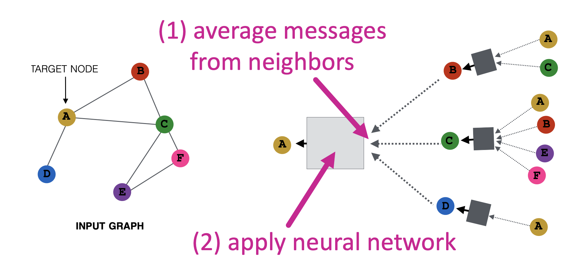Message Passing (see source here) The “messages” are embeddings of a node (at a particular depth) and they are “passed” to their neighbors through a neural network with learnable parameters.

To learn the parameters, we need a loss and some labels. There are a few options.

Explicitly use the product interaction data (the adjacency list). The positive examples are then pairs of nodes that are directly connected. This restricts the meaning of being close as being 1 hop away. Note that a node still gets messages from other nodes that could be more than 1 hop away (Depending on how many layers are there in the NN)
Collect a few nearby nodes by running some flavor of weighted random walks of fixed lengths that start at a particular node. The positive labels are now pairs of nodes that are in the neighborhood of the target node.

After collecting the positive labels, we need to get negative labels. The idea is to sample nodes that are far away from the target node. For large graphs, we can just sample from the uniform distribution and get such nodes with a high probability. These are considered easy negatives, as they are likely to be very unrelated to the target node. However, we want our embeddings to be more discriminative than just being able to separate cameras from bedsheets. So we collect a few hard negatives. Check out the Pinterest’s PinSage for how and when to add these hard negatives.

Here’s a rough outline of what the training loop looks like for the toy graph shown below. I’m going to consider that our positive labels are directly connected nodes. 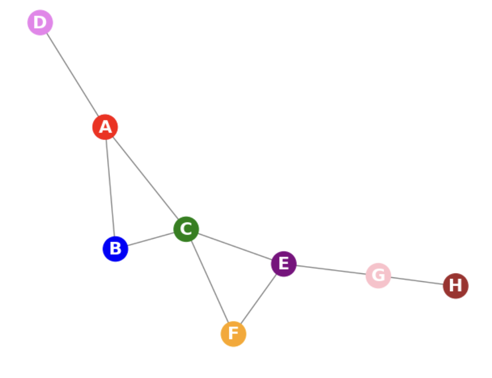A toy graph

Let’s assume that we use a 2 layer Neural Net. The embeddings of all nodes are initialized with product text or image embeddings.

Let’s take [A, B] as the positive label and [A, H] as the negative label. The positive label is a directly connected edge and H was chosen from the background distribution. I’ve conveniently taken a faraway node!
For the forward pass, we sample a subgraph that is rooted at [A, B]. Since we use a 2-layer NN, we limit our exploration to nodes 2 hops away from either [A, B]. When we sample edges, we could use edge weights, node visit counts when running random walks, or some other strategy. One possible subgraph is shown below, where we dropped node F. Note that G and H are more than 2 hops away and hence were never considered.
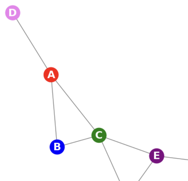Sampling nodes rooted at [A,B]
The forward pass, runs the iterative message passing for each of the nodes shown in the above figure.
We construct the loss from the positive and negative labels. Options are either the logistic loss or max-margin loss.
We back-propagate the loss and adjust the parameters of the NN.

After training, to get the embedding at layer 2 for each node, we run the forward pass for each node in the graph. The PinSage paper has details of how to do this efficiently without having to duplicate computations. To get good embeddings, the negative sampling strategy we choose is crucial.

One major advantage the Graph Neural Network-based recommendations have over word2vec is that we can get recommendations for new products (aka cold start). When a new product enters the catalog, we already have its Layer 0 embedding (using product text or image). We just need to connect this new node in the graph to a few neighbors. A simple thing to look at nodes with similar layer 0 embeddings and make connections. With the parameters we learned we then run the forward pass around the new node to get its layer 2 embeddings

Putting it all together - Personalization, Utility and Rules

So far, our recommendation strategy has just been looking up the most similar product vector for a given query product. Vector search libraries like HNSWLib and Faiss are great at doing this very fast. However, there is a little more work to be done, before we show the recommendations to the user. There are a few things we haven’t considered yet

We haven’t personalized the recommendations to the user. Although for the related products page, the query product is the most important input, it usually helps to add other signals like the user too.
Sometimes we get recommendations that are far away from the product taxonomy of the query product. This could be either due to “noisy” co-occurrence patterns, popular products getting oversampled, etc. We need some filters around product taxonomy to keep things clean. Even if a few people look at woodworking books and wooden shelves in the same session, platforms do not want to recommend these together.
Retailers want to rank recommendations by some notion of utility. This means looking beyond only expected interaction rates. Product margins, promotions, shipping costs, preferred suppliers, etc all enter the mix
Promotions, holiday deals, and the like are used in an ad-hoc way to change the order of recommendations.

Here’s how the components line up. 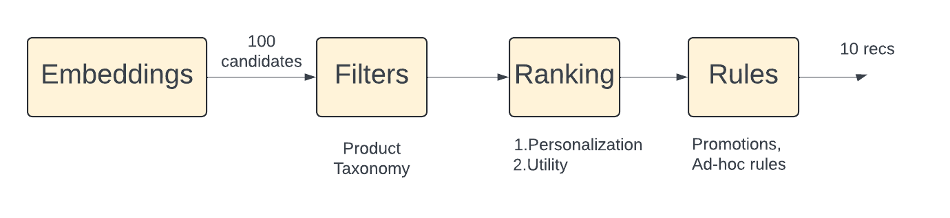Recommendations are more than just embedding similarities

I’ll only briefly talk about the Ranking stage. For the related product strategy, we usually use a lightweight ML model to (re) rank the candidates from the embedding lookup stage. The heavy lifting is already done in the embedding generation stage. For a more detailed look at ranking for ads, please check this earlier post.

Some features that make sense for the lightweight ML model.

Features that capture the similarity of the recommended product to the query product in terms of price and “quality”.The recommendations should be priced similarly to the query. For accessories, this gets interesting.
Features that enable personalization. We can look at the user’s recent interactions to come up with a vector. If the vector is in the same embedding space, a dot product between the product and user vector is a good feature for personalization

To train, the (re) ranking model, logistic regression where we use clicks and impressions (as binary labels) to predict click-through rate and then rank by that probability is the standard approach. This probability if well calibrated can also be multiplied by profit margins or price to maximize expected revenue.

Pitfalls in Evaluation

When working on a new “algorithm”, it’s very tricky to measure its effectiveness. There is already an “old algorithm running”, and all user interactions are influenced by these recommendations.

For offline evaluation, we can train the model on some historical sessions and measure the hit rate on recent test sessions. But remember that the users in the historical sessions can only interact with what is recommended by the “old” algorithm. This feedback loop means that the hit rate only measures how similar the new algorithm is to the old one. There is no way around this problem and we use offline evaluation only to weed out the really bad choices. For example, we can experiment with different negative sampling ratios in word2vec to rule out certain configurations if they have very poor hit rates.

For the online A/B test, we want to take a few versions of the same algorithm (with different hyperparameters for example). However, the feedback loop continues to bite us and make measurements difficult.

Typically we only allocate a small percentage of traffic (say up to 20%) to the “new” algorithm being tested. This means that the “old” algorithm builds its model from the 80% of data that it generates itself (users interact with recommendations to generate the sessions that are used to train the model)
The “new” algorithm is at a disadvantage because its training data is mostly (80%) coming from the old algorithm.

When running A/B tests, this means that as traffic is ramped up to the new algorithm, its metrics (like CTR) could improve. Unless the new algorithm shows a severe drop in metrics, we usually ramp up the test to 50% and keep it running for a couple of weeks to get a better reading of its performance.

Closing thoughts

The recommendations of the Product Page are the most important for any retailer. We talked about a few different ways, the Related Products strategy can be implemented. Graph neural net models are considered state-of-the-art but this is where even naive algorithms can work very well. Even non-personalized best sellers (in that product sub-category) provide a very good baseline model. Measuring the effectiveness of recommendations is also a challenging problem but is well worth spending time on since the payoff when we get things right is huge!