Image classification in the (real) Wild

Posted Aug 9, 2023 Updated Sep 14, 2024

By satyajit gupte

13 min read

Last time we looked at how to best utilize a GPU when training Deep Learning models. Now it is time to put that to use and build a model that can tell apart the bewilderingly similar looking species of flora and fauna. This kind of image classification is generally called Fine grained visual categorization and take a look at these two very similar looking but different species of dragonflies to get an idea of what the model must learn.

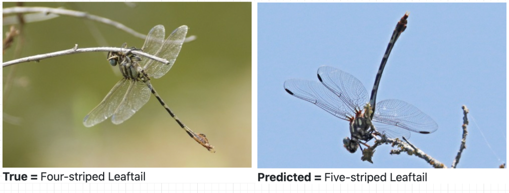_Figure - The Four-striped vs Five-striped Leaftail. The model could not see the difference. Can you ? _

This is definitely not your dogs vs cats intro to CV !

How is the data generated
Building a baseline model
The Recipe
Butterflies are easier than rabbits
Does the model learn Taxonomy ?
An idea for a loss that encourages Taxonomy
Adding Location and Time
How tough is this dataset
Further Reading

How is the data generated

The data comes from iNaturalist, which is an app I use quite a bit. I think it’s one of the best applications of computer vision applied almost directly in the “wild” to make a cool product . Anyone can snap a picture of any living ( or once living) thing and a passionate community of citizen scientists pore over these geolocated images (observations in iNaturalist) and sort them into their correct category. There are over a 100 million observations, including some really rare ones that have helped scientists better understand how a species is distributed.

Building a model with these “labels” and images was a natural progression and now iNaturalist provides suggestions each time you upload an observation, which are most often uncannily correct.

A few years back, iNaturalist opened up some of their data and ran a kaggle competition. The dataset has about 2.7 million observations for 10,000 distinct species. This is the dataset I used.

Building a baseline model

I decided to use the classic ResNet-50 model architecture, initialized with ImageNet weights for the baseline, mostly because I understood it well. I did consider using one of the newer EffecientNet or RegNet flavor of models, but decided to stick with something I had used earlier. Interestingly I wanted to try out a new training “recipe” that the folks at Pytorch claim to have improved the state of the art for all models. I will talk a bit more about this recipe later, but first lets dive into the results.

The model got to about 77% accuracy in 16 epochs. Every epoch took about 3 hours on the T4. Looking at the loss and accuracy curves on the test set, I think the model still had a lot of headroom.

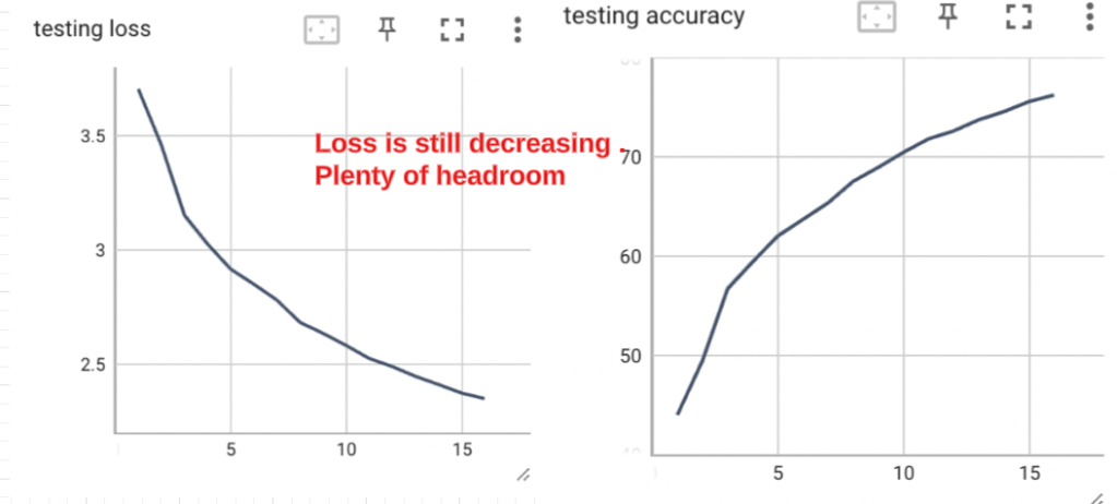_Figure - I stopped at 16 epochs. _

Here’s a look at the model in action. It gets the predicted class ( a Hooded Warbler) right and looking the the Grad-CAM heatmap, it appears that the model thought that the conspicuous black throat and yellow belly were important clues.

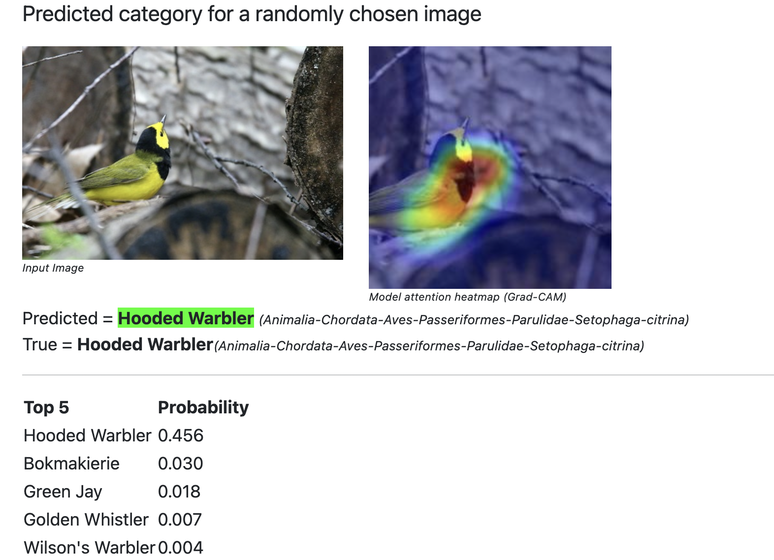_Figure - Looking at what the model predicts _

The Recipe

A lot of the buzz in DL tends to focus (quite understandably) on new model architectures. Not a lot tends to be written about the dark arts of tuning hyperparameters beyond the usual hat tip to some sort of grid search, which is basically trying out a whole range of values to see which does best on your data. This is expensive and with every epoch taking 3 hours, something I did not want to do.

However, the exact choice of these hyper-parameters makes a huge difference in final model accuracy and I ended up using some of the ingredients from this recipe that the good folks at Meta had come up with. They apparently did all the expensive grid search for all of us and provide the magic numbers ! The only kink is that one of important ingredients is training for 600 epochs, well beyond the reach of most of us. However , I still think it’s worthwhile to look at some of the other ingredients.

Vanilla SGD with momentum. The claim is that other more advanced optimizers did not provide any benefit. The last time I did CV, the Adam optimizer was considered the “default” choice, so this is interesting.
Learning rate policy. Learning rate is usually the most important hyper-parameter in any DL model training and getting it right means faster convergence and bypassing the truly treacherous bits of the loss landscape . The recipe increases the LR for the first five epochs linearly (warmup) and then decreases the learning rate smoothly using the cosine function. This is what it looks like .

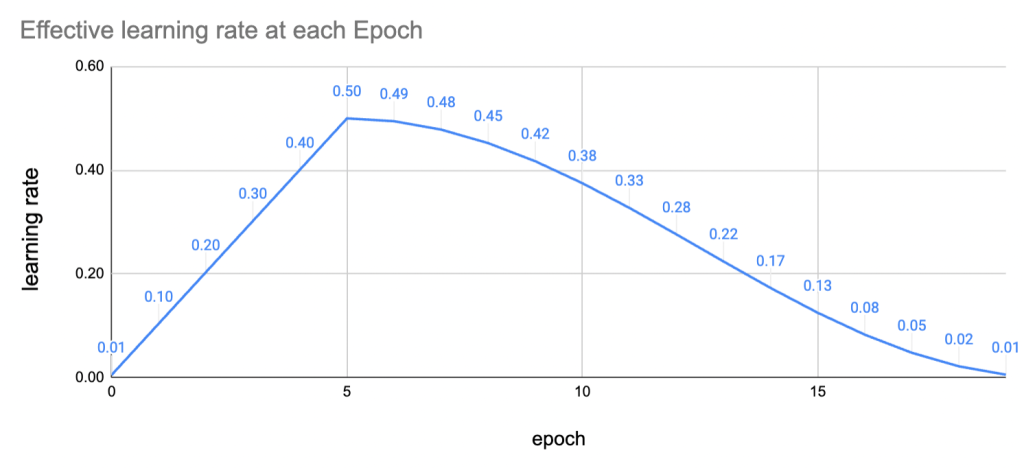Figure - The warmup uses quite high learning rates

Auto Augment. Instead of focusing on only one data augmentation strategy like image rotations or color transforms , this policy chooses one randomly from a whole basket of options like Image shearing, rotations, and a bunch of color transforms. Once an operation like “rotation” is randomly chosen it’s strength (ex angle of rotation) is also randomly chosen. All this means that we don’t have to worry about setting any parameters ourselves.
Label Smoothing. It helps to add a little bit of noise to our labels. After all, even human experts are never 100% confident that thier identification of a Russula species of mushroom is correct, without a DNA sequence. Instead of using hard 1’s and 0’s for the correct and incorrect labels, we simply use a number close to 1 and 0 in the cross entropy loss. This works as a regularizer.

This post by the PyTorch folks has all the details, but it’s good to take a step back and understand that the accuracy gains are only unlocked when training for 600 epochs. I think the theme is that with all the extra regularization (data augmentation, label smoothing, etc), we need to train for much longer. What we do end up with is a much better model and all these hyperparameter choices help unlock these gains.

Butterflies are easier than rabbits

Visually inspecting some of the model errors is one of the most useful ways to spend time debugging the performance. The species are all classified in a hierarchy and I found it really useful to see which groups had higher and lower than average accuracy.

Here are some groups that the model did considerably worse than average.

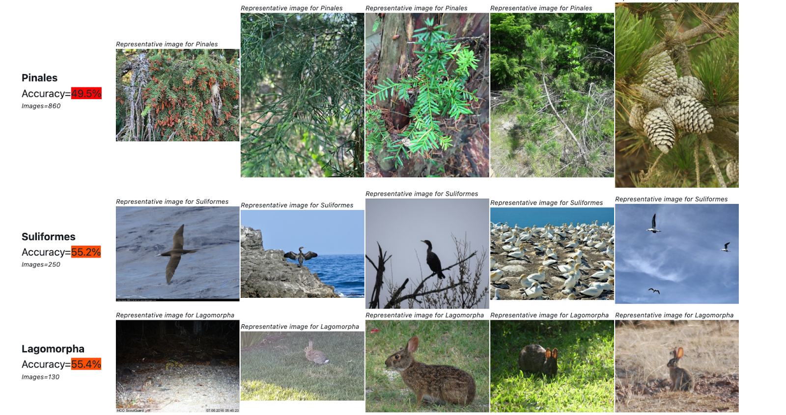_Figure - Groups with lower accuracy. _

Latin taxonomic names always throw me off and I had to look at some of the images to see what exactly is a Pinales (they are Pine trees), or a Suliformes (water birds like cormorants)

Lets now see what groups the model did rather well on

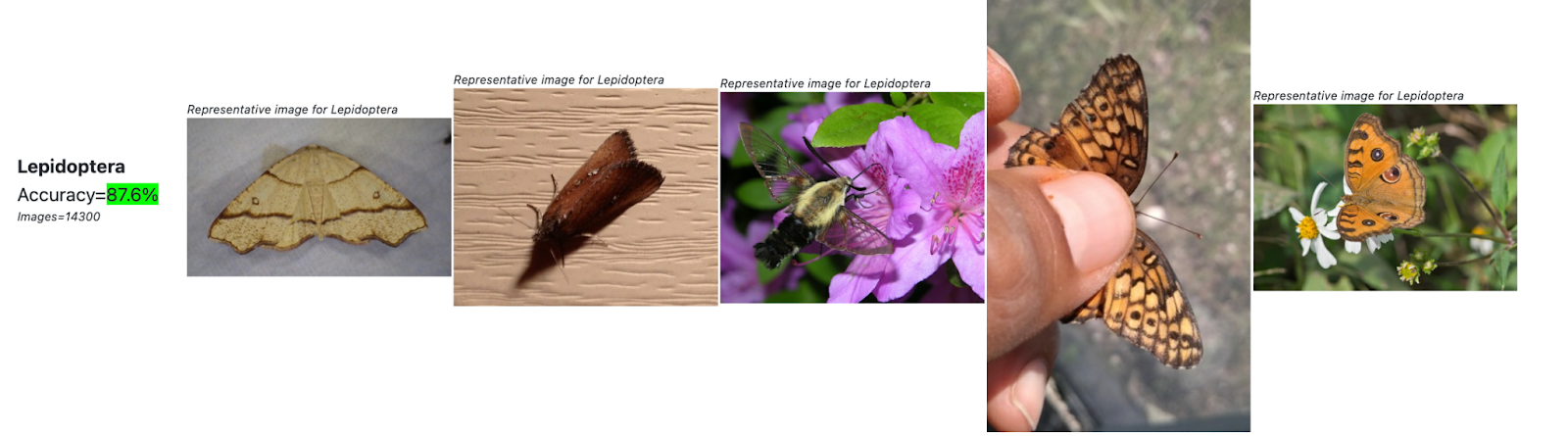
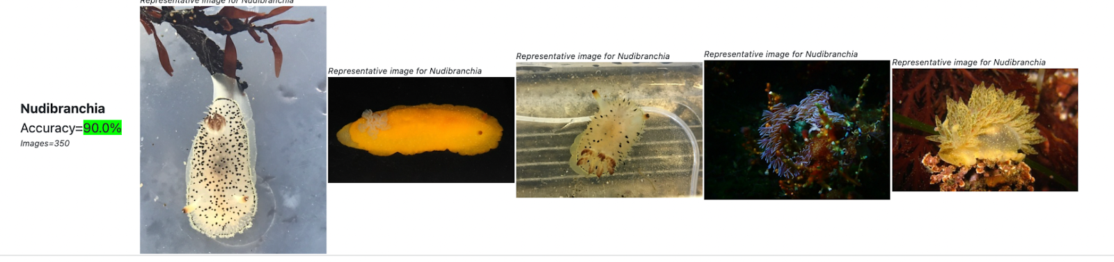_ Figure - Butterflies and sea snails are brightly patterned and have higher accuracy_

After spending quite some time looking at metrics and images like these , I think some themes are notable.

The model does well on strikingly patterned groups like butterflies, sea snails and beetles
The model struggles on groups that are not so visually sharply defined. A long shot of pine trees or a perched cormorant does not provide enough clues. All rabbits (lagomorphs) are brown furry balls.
Perhaps, there is also a bias in what images are uploaded. I would hazard a guess that most folks who are into butterflies or sea snails, usually take good close up photographs. Shore birds and the like are just more difficult to get close to.
I believe even experts would want to look more closely at groups like pine trees, before passing judgment. Fine details like how the bark is patterned (I’m thinking about Ponderosa pines) or how the pine needles are bunched up are used to get to the right species.

I also looked at some of the model errors at the top of the taxonomic tree. Its obviously much worse if a plant is incorrectly called an animal as compared to calling a eurasian curlew a long billed curlew.

Here are some incorrect classifications at the Kingdom level.

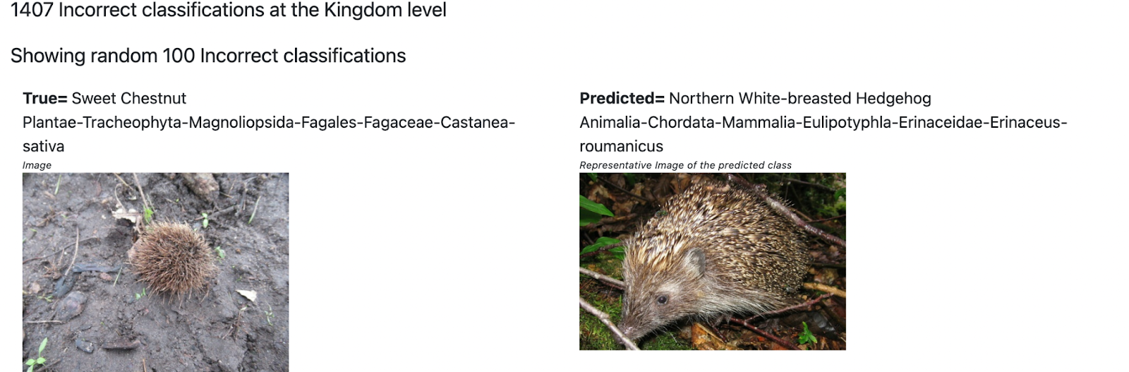Figure - Mistaking a bush for a hedgehog !

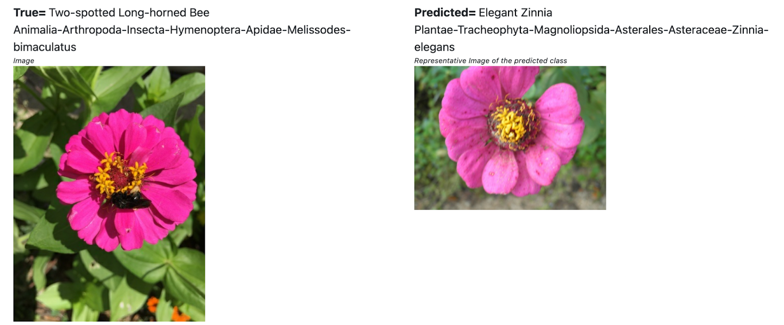Figure - a bee on a flower. Whats the correct id ?

In the first case, a spiny looking shrub is incorrectly classified as a hedgehog. I found this quite funny !

In the second case , the image has a bee perched on a flower. The “true” label is the bee, but the model calls it a flower. I noticed quite a few such cases when grouping the errors at the Kingdom level. I would not fault the model for this.

Here is another interesting error.

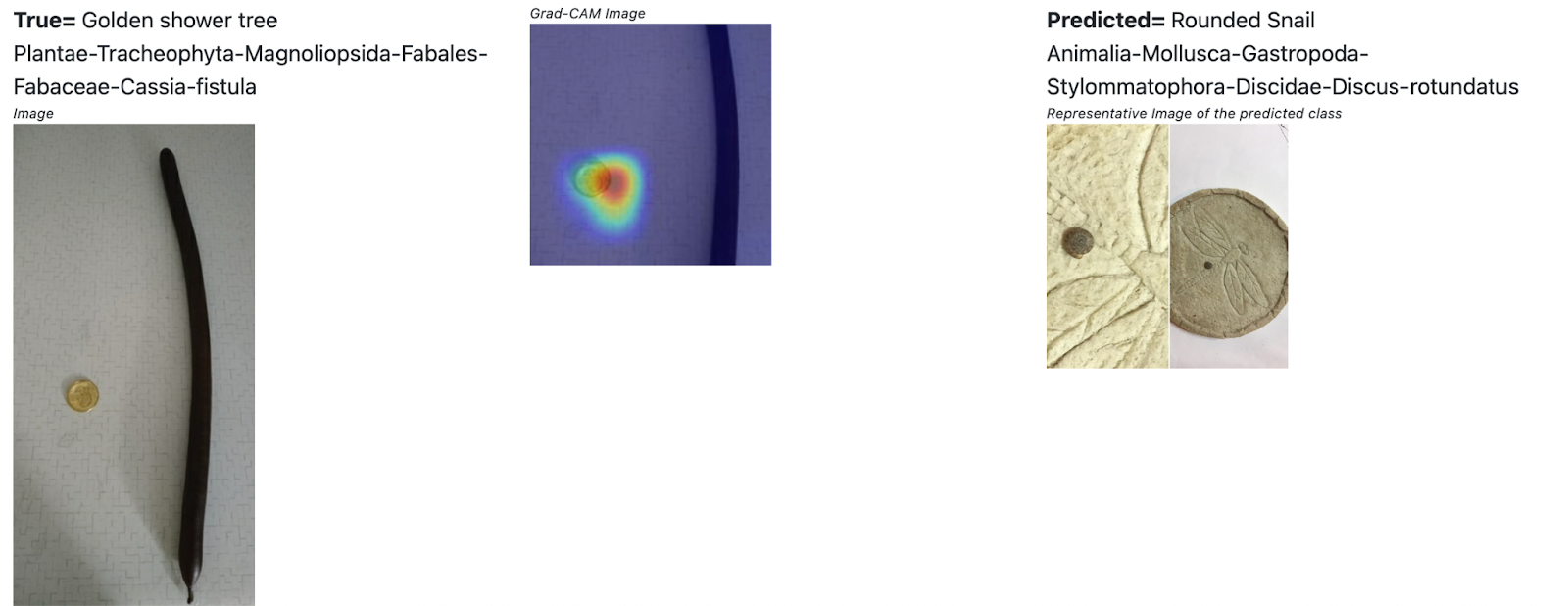_Figure - A coin placed for size reference, throws the model off _

The observer has placed a coin for size reference (a common practice) next to what looks like a branch of a tree and the model focuses on the coin to classify it as a snail. I think what’s going on is that a lot of the snail images have coins for size reference. This is an interesting visual artifact that the model learns to associate with certain classes. I don’t think models like Resnet learn to use the coin as a size reference as humans would.

Does the model learn Taxonomy ?

The Linneaus system of classification is what we all learned in school. Although it now looks a little frayed at the edges thanks to cladistics and genetic sequencing, its time has not yet come.

In our classification model, we treat all the 10,000 classes as distinct categories and biologists probably sneer at such stupidity.

We did not use any notion of taxonomy in the model and I was curious to see how the model errors were distributed.

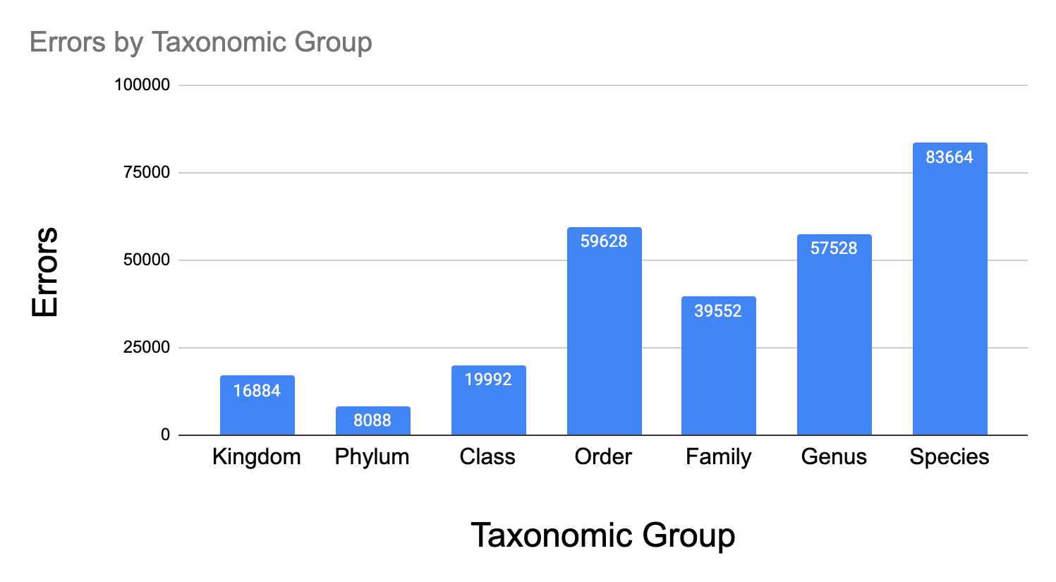
Most of the errors (~33%) are at the species level and the shape of this distribution looks reasonable. In Spite of the higher error under “Order” and “Kingdom” , I think the model does learn something about the taxonomy. Another interpretation is that the Linnaean system of taxonomy roughly matches visual groupings.

Most of the errors under Order look like mis-identified plants and birds

An idea for a loss that encourages Taxonomy

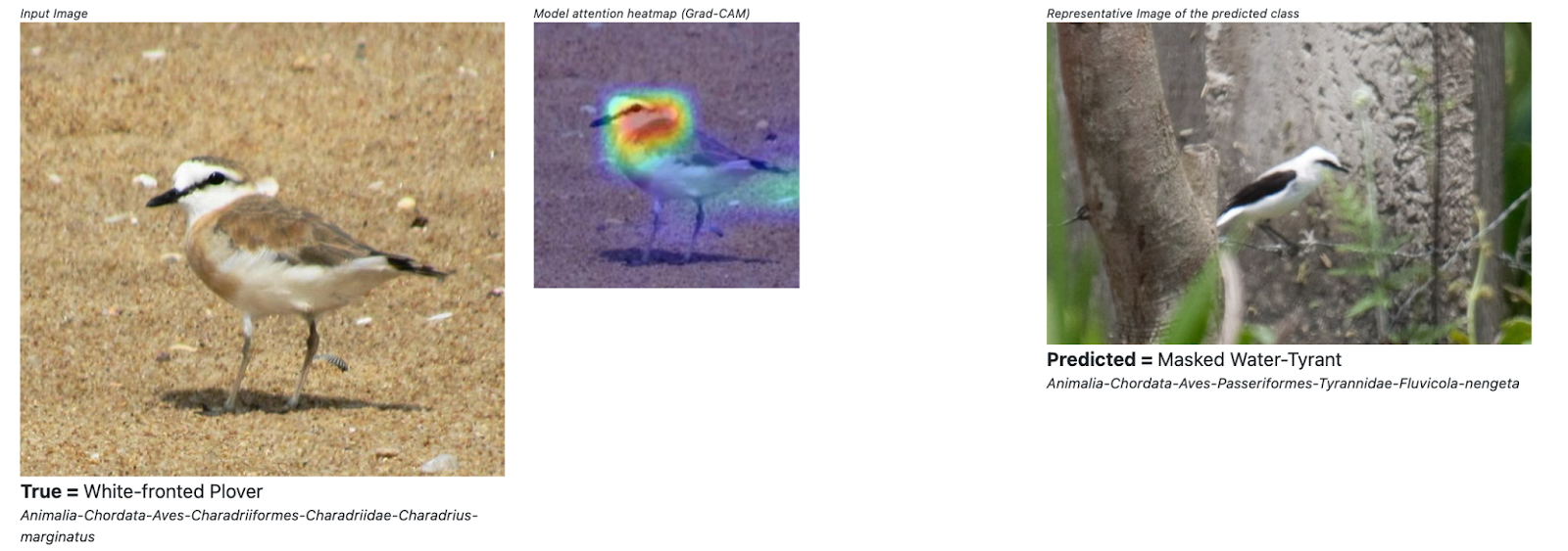
Looking at some of the misclassifications I think it might be worthwhile to try out a custom loss function that penalizes some errors more than others. One way to quickly try this out could be to use a similar idea as the label smoothing technique, but smooth only over “nearby” species. For example, for a particular bird, say a White fronted Plover, we smooth progressively over the same Genus (all Plovers), Family (plovers, lapwings) and so on. How far up the hierarchy we go and how to decay the smoothing would all be hyper-parameters to explore.

It’s possible that a model with this loss function does slightly worse at species level classifications, but improves the shape of the error distribution across Taxon groups. Something to experiment with in the future !

Adding Location and Time

In the baseline model, I did not add location and time as features. Pick up any field guide on birds or butterflies and you will see a section on geographical range and seasonality, so these are going to be important features. As every birder knows, a brown babbler, is much more likely to be a yellow billed babbler if found in southern India. It looks very similar to the Jungle babbler which is more widespread elsewhere.

I wrapped the latitude and longitude in trigonometric functions so that they wrap around the earth and fed them into a shallow neural net with a few Fully connected layers. I Concatenated the output of the last layer in the ResNet ( dimension = 2048) with the last layer of this “GeoNet”, followed by another Fully connected layer that should learn how to best combine image and geo-location.

This model did have higher test accuracy in the first few epochs, but the accuracy dropped and loss increased after the 3rd epoch. My hypothesis is that the learning rate policy with warm up sets the learning rate too high (around 0.3) for the shallow Geo Net. The ResNet is a deep conv net and using the same learning rate for a shallow network probably causes the shallow “Geo Net” to diverge. The fix would be to scale down the learning rate for the shallow network and PyTorch does provide easy ways to do that. I did not experiment with this though. I instead just slapped on GeoNet on the baseline model (already trained for 16 epochs using iNat data) and trained for 2 epochs. This model got to about 80% accuracy.

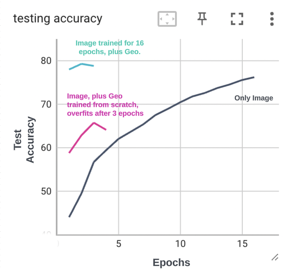Figure - Test accuracy

I then read about GeoPrior a model that encodes location and time to learn priors for species. This seems like a very nice way to basically combine priors with any kind of classification model. This is something I want to explore more. However my guess is that with the right learning rate for each subnetwork a combined model learned jointly end to end should do better than learning separate models and then multiplying their output probs.

How tough is this dataset

Looking at the accuracy of this model and looking at the kaggle competition winners (they got close to 95% accuracy) got me thinking about the toughness of this problem. For context the state of the art on ImageNet is around 85% and ImageNet only has 1,000 classes. How is it that with 10X more classes (which are more fine-grained), these models apparently get such good accuracy. The authors of the winning model claim that location added +5% to the accuracy so there is something more going on. I do not have a good answer to this question right now.