How Ads Work - Part 3, Ranking

Posted Mar 10, 2023 Updated Sep 14, 2024

By satyajit gupte

20 min read

Welcome to the third post in the How Ads work series. In this post we are going to discuss Ads Ranking in depth. This is where ML really comes to the party! At the end of Ads Retrieval, we have a pool of about a thousand fairly relevant ad candidates. Now it’s time to really identify the very best ads.

Formulating it as a ML problem
Training Data
Model Evaluation Metrics
Models
How to Train and Test the model
Continuous Training
Model monitoring
Logging pipeline
Feedback Loops
Other Ranking Models
Ranking Utility
Closing thoughts
Further reading

Formulating it as a ML problem

Our goal is to find the most relevant ads. We are going to use a click as a proxy for relevance. Now the problem becomes predicting clicks and ranking the ads by the probability of getting clicked. We can frame this as a binary classification problem, where a positive label (y = 1) is when an ad that was shown (impressed) was clicked and a negative label (y = 0) is when an ad was shown and not clicked.

Formally, we want to predict prob(ad clicked when ad shown). Let’s call this pClick.

If ranking is all we cared about, as long as the ads are sorted by pClick, we would be done. For ads though, in the Auction we want to estimate the expected revenue by multiplying pClick by the bid. So we want pClick to be calibrated too. Ads have advertiser budgets and if pClick were to be systematically higher (or lower) we run the risk of exhausting (or not using up) the budget. Well calibrated predictions keep the Auction efficient.

Training Data

Our training data is going to come from historical user clicks on ad impressions. This gives us a large volume of data and we can happily build complex models. One thing to keep in mind is that click through rate for ads is very very low (< 1%). So this is an extremely unbalanced dataset and trying to train a model directly on this is not a good idea. The fix is to downsample the negative (y = 0) class by a factor of 10 or so. This gives us a much more balanced ratio of positives to negatives.

We use a time based split to create the train and test sets. Usually , we use several weeks of data to train, and then use the next day to test. To really mimic how the model is used in production, we can also create a rolling train & test split. We will discuss this in depth later.

It’s also a good idea to see if there are some very unusually active users in our data. If so, we can cap the number of impressions per user. This prevents the model from overfitting to a few highly active users.

Model Evaluation Metrics

Since we framed the problem as a binary classification problem, we are going to be optimizing for Log Loss (aka binary cross entropy)

Normalizing the log loss by the entropy of the empirical click through rate (CTR) is an even better metric, as it measures the relative improvement over just predicting the empirical CTR.

\[Normalized Log Loss = \frac{-\frac{1}{N}\sum_{i=1}^{N} y_{i}*log(p_i) + (1-y_i)*log(1-p_i)}{-(p*log(p) + (1-p)*log(1-p))}\]

where p (in the denominator) = empirical CTR

AUC is also a good metric to track, but it only captures the relative ordering of ad scores. To track how close the probability estimates are to the empirical CTR we measure calibration. Calibration is the ratio of the average pClick to the empirical CTR

$Calibration = \frac{\frac{1}{N}\sum p_i}{p}$

So the metrics we track are

Normalized Log Loss. Lower the better.
AUC under the true positive rate (tpr) vs false positive rate (fpr) curve. Higher the better.
Calibration. The closer it is to 1, the better

Models

Our strategy will be to optimize for LogLoss and Calibration in two separate models and then use a cascade of two models. The first is a Deep Learning (aka DL) base model where we plug in a whole lot of features. The goal of this model is to optimize for Log loss. DL models are known to be poorly calibrated and to fix that we have the second model which is a simple Logistic regression model which takes as input the output of the DL base model and a few other features.

The base DL model is large and could have hundreds of millions parameters. It is trained on a very large amount of historical data (several weeks) and then frozen. The calibration model takes only a handful of features and is trained on a much smaller amount of data (a few hours). Take a look at the model structure in the figure below.

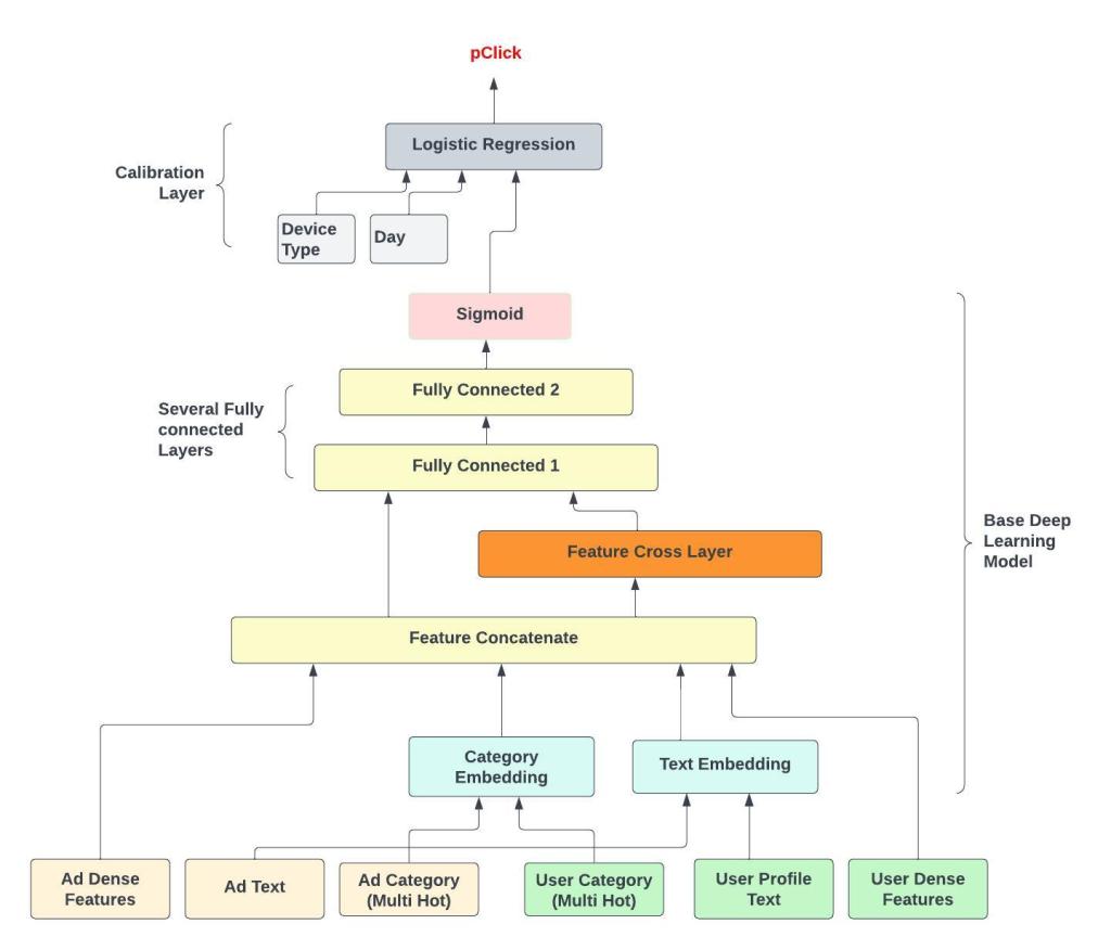Figure - A cascade of two models (only a few example features shown)

Features for the Base Model

For the base DL model it’s useful to group the features semantically into User, Ad and Context. Here is a small sample of features that are used.

Ad Features

Ad and Advertiser ctr for last 7 days, 30days. These historical features are usually the most important features. The past is sometimes the best predictor of the future !
Ad Id and Advertiser Id. One Hot and Hashed into a fixed size Vocabulary. These help the model memorize patterns specific to a particular ad.
Keyword tokens from the Ad title, description, landing page.
Category and topic inferred for the Ad. Usually multi hot sparse vectors.
Embeddings based on Image or Text. These embeddings can be learnt in a previous ML pipeline.
Ad type. The Ad could be textual, image or video for example.

User Features

Historical user interactions with the Advertiser, Ad category, etc
User demographics and profile like gender, geographic location.
Category and topics that the user is interested in. These could be inferred by other ML pipelines.
Uer embeddings . A simple way to generate these is to take an average of the last few interacted ad or organic embeddings.

Context Features

Device type and day of the week
For search ads, we also have tokens from search query.

Special features

Position. User’s click a lot more on higher slots. So where an ad is displayed has a major impact on its CTR . This is a great explanatory feature to be used in training. During online serving , we set this feature to 1 every time. This removes the position bias and means that we actually predict the pClick for the 1st slot for all ads.
Age of the Ad. How old the ad is also an important explanatory feature, Similar to position we use it during training but not in serving.
Retrieval candidate source. Remember that in the previous stage of Retrieval, there are usually several candidate generators. Some of these (ex the Two Tower model we discussed in depth) will give more relevant ads than others. We can use this information as a feature. However we should not use any scores from retrieval as those are usually not comparable between different candidate generators in retrieval.

What to do when features are missing

Both during training and serving, we don’t expect every feature to be available for every example we want to score. Some features are generated using other ML pipelines and may take a while before they become available for a new Ad. Sometimes, the user might have profile and demographic information missing. A good way to handle these cases is to add a binary feature that indicates if a particular feature is missing. For example for the ad embedding we add another feature is_ad_embedding_missing that is set to 1 if missing and 0 otherwise. Note this is much better than just using the default value for these vectors (which is 0 usually). Explicitly creating an indicator binary feature helps the model a lot.

When a feature is missing, we set its is_missing indicator feature and use a sensible default for its feature value. Using an average for numeric features and a special Id for One Hot or MultiHot as default values are good ideas.

Feature Preprocessing

We can group these features is into One Hot, Multi Hot, Numerics, Text and Dense Vectors to see how preprocessing is usually done. Feel feel to skip this section if you already went through the Ads Retrieval post as it is similar.

One Hot and categorical features are hashed into a fixed dimension vector and then fed into an embedding layer. This embedding layer can be shared between the Ad And User for the same feature. For example the ad and user category multi hot vectors can share embeddings as long as the category Ids mean the same thing for both the Ad and User.

Numerical features are normalized to be within a small range like [-1, 1] . Typically we use z-score normalization. If the distribution of the feature is heavily skewed, we can instead use quantile binning to convert it into a categorical feature. Adding feature transforms like taking square root, powers or log also usually helps. These simple small nudges surprisingly help even cutting edge DL models.

Text strings are tokenized and hashed into a fixed size Multi Hot vector. Embeddings for each token are learnt and then an averaging layer summaries all the information into a single dense vector. We ignore the order of tokens in this approach.

Most ads have an image. We can generate dense embeddings from these by passing through an Imagenet like model. Or better still have our own fine tuned visual model trained on some domain specific task. For the purpose of the Ranking model we can think of these other models simply as pre learnt feature transformers.

The Layers in the Base Model

The initial layers are embeddings for MultiHot and One Hot Vectors and Preprocessing layers for Dense and Numeric Vectors.

After we concatenate everything into a nice big vector, we do a full feature cross. The feature cross layer is simply the input vector multiplied with its own transpose. The matrix that results has all the possible pairwise feature interactions. In theory Deep Learning is supposed to learn these sorts of interactions, but doing this explicit crossing greases the wheels a lot.

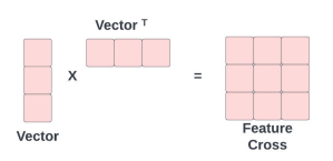Figure - Feature Cross Layer

The Feature Cross Layers does not have any parameters to learn. We flatten the result and feed it into the Fully Connected Layers that follow. It’s a good idea to follow every Fully connected layer with BatchNormalization and Dropout. The top most layer is a sigmoid.

The Calibration Model

Once the base DL model is trained (AUC and LogLoss look good), we freeze it. It’s a good idea to check how mis-calibrated the base DL model is. There are two reasons why the calibration of the base model is poor.

We downsampled the negatives. This would have been easy to fix by simply scaling the output . We don’t bother with scaling the output because the calibration layer should easily learn this.
DL models are known to be mis-calibrated. The calibration layer is a simple fix for this.

The calibration model is a simple Logistic regression model that takes as input these features

The output of the base DL model
A handful of context features like device type, day of the week, etc. We choose these features to give the calibration model a bit of flexibility in learning how empirical CTR varies for these important context features.

The calibration model should not affect the AUC. In fact, if we only use the output of the base DL model as the input feature, it is guaranteed to not change the AUC of the base model, as we only monotonically transform the score. This calibration technique is also called Platt scaling. Plotting a calibration curve like in the figure below will show you regions where the model is over and under calibrated. To draw this plot, we bin the predictions onto equal sized bins and then take the average predicted value in each bin (x axis) and plot it against the fraction of positives (ad click , y = 1) in that bin.

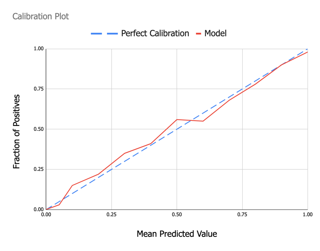Figure - Calibration Plot

How to Train and Test the model

We partition our data into three time separated chunks and train the two models in stages.

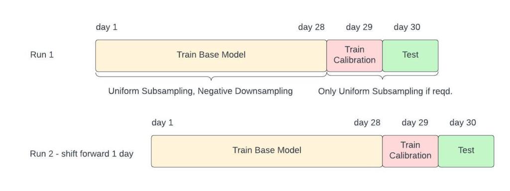Figure - Rolling Train and Test splits, N = 28 in this example

Train the base model with several week(s) of data. Call these days Day 1 to Day N. We subsample the data uniformly (if required) and do negative sampling on this set. Sampling rates are a parameter we need to tune.
Once the base model converges, freeze the base model. We sanity check the base model by measuring metrics on the test set. We expect calibration to be bad.
Train the calibration model on a single day’s data. This day should be Day N + 1.
Measure metrics on the test set, which is Day N+2.
Repeat the whole process, after moving one day ahead, We do this for at least 7 days, as we want to check model performance especially on weekends, when users seem to suddenly go click happy.
Finally we can average out the metrics over 7 days to understand overall performance

This scheme might appear to be a bit complicated, but remember that many Billions of dollars flow through these Ad Ranking models. It’s definitely a good return on investment to evaluate the model thoroughly.

Continuous Training

Ads are created and die out very fast. New Ad campaigns are launched frequently and seasonal sales can affect user behavior very rapidly. Tracking how metrics deteriorate when you use really old data to train, should quickly convince you of this. Training the base model once a day should be fine, but we definitely should aim to train the calibration model at least hourly.

Train the base model once a day, using the last several weeks of data. We don’t need to randomly initialize the model each time. Using the last model as a starting point is a good idea as long as we haven’t introduced any new features.
Train the calibration layer, every hour using data from the last 24 hours. These numbers are just rough guidelines

Finding out how much data to use to train the base and calibration model is something that we should spend time experimenting with. Plotting how the metrics improve and eventually plateau off with additional data will tell you how much data is required for each model.

What I have described here is basically batch training. Truly online learning, where every new label changes the model is tricky to get right and might not provide enough value.

Model monitoring

Since we have a model that trains continuously, we need some checks before we can start using it on live traffic. If any of these checks fail, we simply use the last trained model and can investigate why this model messed up at leisure. The checks are of two kinds.

Offline checks. Have bounds for dataset sizes, calibration errors and AUC. Suddenly less data, or wacky metrics are a sign that something broke.
Run some integration tests with recent (but not live) traffic. It’s simple to measure shifts in click probability distributions. With a little bit of plumbing, we can join the recent impressions with clicks, to measure AUC and calibration on very recent user data too.

We also have monitoring to check for feature coverage, drifts in feature distributions and a bunch of other things. There is a lot more here that we will skip over.

Logging pipeline

When we talked about training data, we glossed over a lot of details. It’s time to peek a little more into the mechanics of how training data is generated.

When user’s view ads, we get a stream of impressions. Every ad that gets viewed has a unique ID, which we call the ImpressionID. We also log the features used by the Ranking model.

When users click on ad, we get a stream of clicks. Every ad in this stream also has an impressionID.

The Stream Joiner joins impressions with the clicks to give us the training data. Ads that appear in the clickstream are labeled 1 and all other impressed ads get the label 0.

In the picture above, ads a, c and e got clicked by users. Note how the ads can arrive out of order in the clickstream.

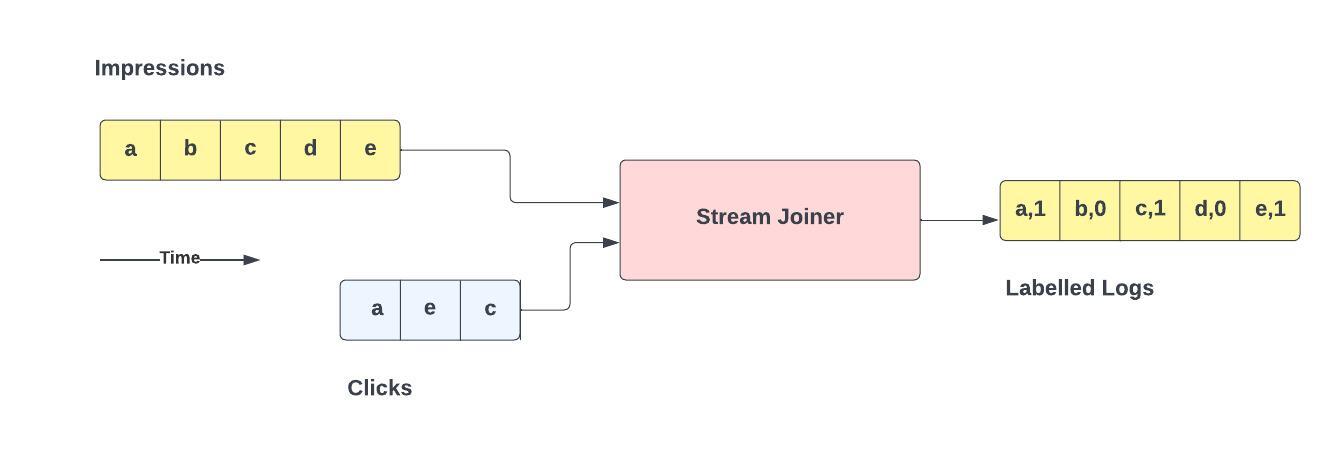
The stream joiner usually maintains a time window, and if an impression does not show up during that window of time in the clickstream, it marks it as not clicked. A side effect of this is that there will be a few ads that actually got clicked but arrived too late to be joined and got incorrectly labeled as not clicked. This means that the true click through rate is a little higher than what we have in our training data and what we trained the model to predict. Measuring this difference, we can scale up our click predictions as a final post-processing step.

Feedback Loops

In the steady state, our ranking model selects the ads that get impressed and clicked. This very same data is used to train our ranking model. This creates a strong feedback loop, which is undesirable, because it can mean that the same (or similar) ads get shown repeatedly. In any model trained on implicit labels, some amount of feedback loop is inevitable , but there are a few strategies to minimize it.

Use position as a feature to train the model, but set it to 1 for all ads during inference
Do not use bid as a feature in the Ranking models. We don’t want the model to learn any patterns around bid.
Add a little bit of random noise to the output of the Ranking model. This comes at the cost of showing poorer ads to the user , so we do it only for a tiny percentage of users.

Other Ranking Models

Ranking ads only by click probability can lead to a lot of click-bait ads getting shown. Users might click on visually distracting ads that show fat and teary celebrities but after a while, most users get turned off by click bait.

We need some other tools to make sure that ads are truly click worthy. Let’s take a look

Users will spend more time on really relevant ads. Let’s define a Long click as an ad that the user spent at least 10 seconds on.
The UX often gives users a way to dismiss or hide ads that they don’t want to see again. This is an explicit label and although very few users do this, it provides a very strong negative label.

Of course, we are ML people and we can set it up just as we formulated the click prediction problem as binary classification problem. The Long click and Hide prediction models will have much lesser training data and we can either .

Train separate models for each task that are much simpler. So use only the best features and keep the number of parameters down.
Train a multi task (MTL) model . Intuitively we should expect the tasks of predicting clicks, long clicks and hides to be correlated.

I’ll talk about the MTL approach a bit because it is really attractive. It allows us to use data for a slightly different but correlated task and also helps us to keep the model zoo less unruly.

There are two ways we can implement the MTL idea.

Full on MTL , with one large mixed label training dataset and different weights for the loss on each task.
Lite MTL. First train the base click prediction model. Freeze the base DL model and then add a block of a few layers for each task. Learn only the parameters for these newly added layers. Use the exact same features as the base click model.

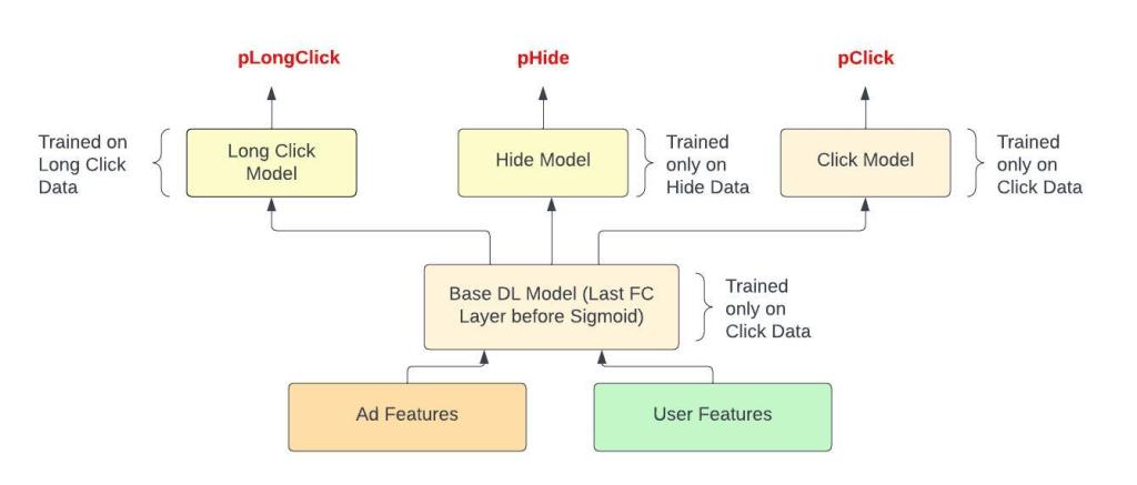Figure - Lite MTL to predict 3 different actions

We will prefer the Lite MTL approach because it keeps things simpler.

We don’t have to worry about how much to weigh each task
Model releases are siloed, and improving the hide model for example is guaranteed to not affect the click model. Remember that the click prediction model is the king of the models and we are quite protective of this.

This Lite MTL approach does come at the cost of not being able to leverage the hide and long click data to improve the click model, but I think this is a good tradeoff.

Ranking Utility

Once we have model predictions for these tasks it’s time to put them together. A simple linear combination is what will do the trick. I believe there is some theory that supports this linear formulation (as opposed to multiplying the scores for example), but we will not go into too much depth here.

Most platforms combine these scores with some weights and compute what is called the Ranking Utility. These weights are usually hand tuned (yay secret sauce !) and the overall goal is to optimize for long term revenue.

Ranking Utility = w1*pClick + w2*pLongClick - w3*pHide

Formulating this as an ML problem, where we try to learn the weights on each prediction is a worthy challenge.

Closing thoughts

We covered a lot of ground in this post. Ranking is where most of the ML action in Ads is. Accurate and well calibrated models are the key to having a healthy platform. In this post, we talked only about Deep learning models. I want to point out that unlike Vision and Text where Deep learning blew out the earlier generation of Machine Learning morls , for Ads, it’s only fairly recently that DL has become the state of the art. Gradient Boosted Decision Trees and Logistic Regression are very strong baselines and are perfectly decent for this task too.

Thank you for reading and please leave a comment if you have any questions.